When talking about scalable data engineering there are four broad categories of questions that we like to start with. I like to call these the four V’s of Good Data Engineering: Volume, Velocity, Variety and Veracity.
Overview
Volume
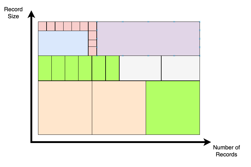
Volume is simply a measure of how much data you wish to process. This is usually a discussion of gross numbers and timelines associated with them, and gives a rough idea of some architecture constraints and guidelines. For volume the discussion is a straightforward one about business goals and aspirations. Usually the discussion breaks down as follows:
Current Volume:
What is the current volume of data that a particular data pipeline or system is processing. You can also discuss the current architecture and any bottlenecks it may be facing. When looking at current volume of data some considerations that may matter are:
- Volumes per access level: What volumes of data currently in terms of access patterns. In other words, there may be 10 PB worth of data, but 9 PB of that may be “cold data” or archive data and only 1 PB is regularly accessed or used for any analytics. Further than that it could be that only 1 TB is “hot data” or data that is frequently accessed. This will also impact how data estimates could be affected, for example archive data may be compressed or stored in columnar or analytical formats which would not give an accurate comparison to row based serial data.
- Data Retention Companies may not be keeping all the data they wish to currently keep and have imposed retention policies which they may choose to remove if they have a more scalable data strategy in place. Data Retention can also be used to estimate the amount of data flowing through a system regardless of persistence for data processing purposes.
- Record/Message size For each current dataset, how big is a record, and at a static point in time how many records of that size are there? In a streaming context this can impose hard limitations on what technologies can be used (Kafka vs. Kinesis for example), in a static data warehousing context it may give ideas about current suboptimal data model design or heavy denormalization patterns along low latency paths in the data pipeline.
- Data Footprint The amount of data a company stores may not be reflective of the total data footprint the company has especially when taking into consideration data retention policies, data that is ephemeral or not stored anywhere, or query patterns which adopt patterns of heavy denormalization. In well-designed systems some denormalization will lend itself towards better separation between write and read latencies, but will result in a lot of duplicate data. Another example of necessary duplicate data is in RAID configurations or replication such as with HDFS, and backups. In other cases there may be unnecessary duplicate data. Its important to suss out instances of heavy data duplication, necessary or not, in order to get a sense for the total data footprint and distinguish between “raw” system data and derived data that the company has synthesized for various reasons.
- Key Datasets It may also be helpful to get a sense for what are the largest datasets a company deals with and the most frequently changing. Sometimes you can infer key elements about how that dataset may change over time, and thus the right strategy for designing around that dataset. For example if they say their largest dataset is “users” and they are a B2C retail company then you can infer that table is most likely to see heavy growth as the business grows, and will have higher demands for read and write latency.
Desired Volume:
What is the volume of data the company “wishes” to be able to process in the system. “As much as possible” is not an option, it must be finite and realistic. Over provisioning data processing capacity can get expensive really quickly, especially on the higher ends. More open-ended needs and requirements around scaling can be approached using autoscaling or adaptive scheduling. If the answer is “we dont know” an effort should at least be made to help the company try to estimate.
Anticipated Volume:
This is meant to bookend the previous point. Whereas as the desired volume is where the company wants to be in X years, the anticipated volume is where the company is most likely going to be within that time. This serves as a lower bound where the desired volume forms a rough upper bound. A less jarring way to discuss desired and anticipated volume (because after all what business is going to admit they aren’t going to grow as fast as they want, even though for most businesses the amount of data being handled is a bad vanity metric) is to simply discuss upper and lower bounds of needed capacity.
Velocity
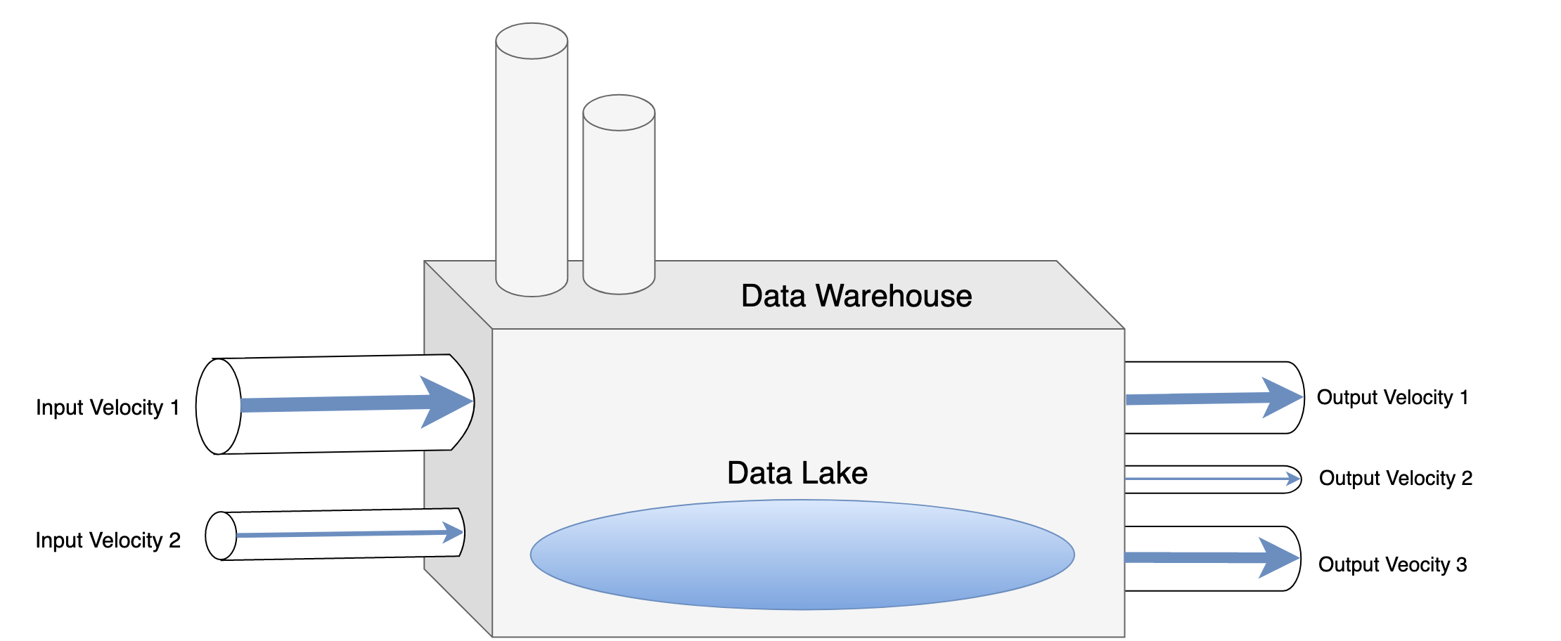
Velocity is a measure of how quickly the data is moving over time regardless of the volume of data. Normally it’s hard to talk about data velocity without talking about its desired latencies or limits of time that you have in order to process the data which is usually imposed by external technical or business requirements. You can talk about roughly 3 types of velocity:
Input Velocity:
How quickly is data coming into the system and how does the system need to accommodate that. This can be as simple as knowing that you only have batch access to the data (daily data dumps) vs stream access to a particular subset of the data, thus can only in best case scenario provide batch analytics on it. Or it can be as complex as planning very tailored distributed stream systems to get a specific input consumption rate.
Output Velocity:
How quickly does the data need to be accessed or read. Typically this is tied to the front end of the process and the business use cases of how the data is being used. Limits on the associated output latency may vary for different subsets of the data, and may also make exchanges between consistency and availability (in the spirit of the CAP theorem). In plain terms, you may be willing to sacrifice accuracy of the data for getting it quicker, or you may opt to scale out further in order to get tighter control over both speed and accuracy.
Intra Velocity
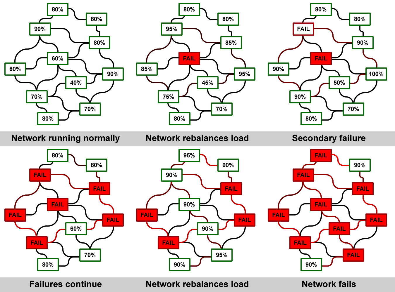
Intra latency is the amount of latency that is permissible between input and output velocity, or you can think of it between the various components of a data pipeline. Intra velocity in a data pipeline is a little harder to tack down. Usually this is either an operational metric, or something that is observed and optimized post-hoc. However, this doesn’t mean it isn’t important as it can have cascading effects on other parts of a data pipeline, sometimes in unexpected ways. In streaming systems back pressure engineering is one way to observe and respond dynamically to changes and levels of intra velocity.
End to End Latency
Putting together the three latencies associated with each of these and you arrive at what people typically refer to as “end to end” latency requirements, ie once a piece of data hits your system, how much time do you have before your analytics or end users will see the impact of that data. Keep in mind that varying business use cases may have varying requirements around end to end latency. It is not a universal metric. However, multiple data pipelines may end up affecting one particular end to end latency and may require you to more carefully engineer a particular pipeline to “keep pace” with other parts of the pipeline.
Pressure
Before going onto Variety, I want to make a quick note about the relationship between Volume and Velocity as they don’t exist in isolation but in terms of planning are heavily dependent on one another. In order to do so I want to introduce the idea of “data pressure”.
You can think of Data Pressure as follows:
Data Pressure = Data Volume x Data Velocity
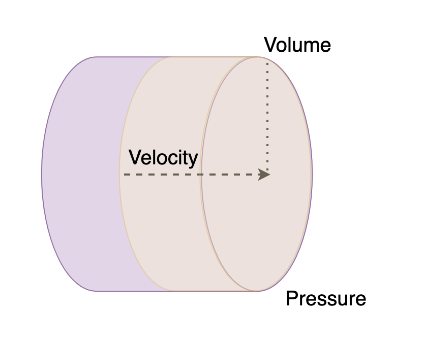
In other words a relatively low desired data velocity might be offset by higher data volume and vice versa. This basically expresses the data volume in terms of total amount of data needed to be processed per unit time. It is interesting to look at the limits of data pressure. For example, a really low data volume but high input velocity may lend itself towards stream processing. However, if the needed output velocity on the opposite end of the process velocity is very low, say daily, then it may lend itself towards buffering and then batch processing. In short, the pressure expresses how much strain is put on particular parts of a system and what extra parts of the system may need to be designed intermediately in order to marry front and backend pressure demands gracefully. Those parts that feel more pressure than may need to be given special attention, for example, horizontal scaling, or other strategies such as breaking up the data pipeline stages differently.
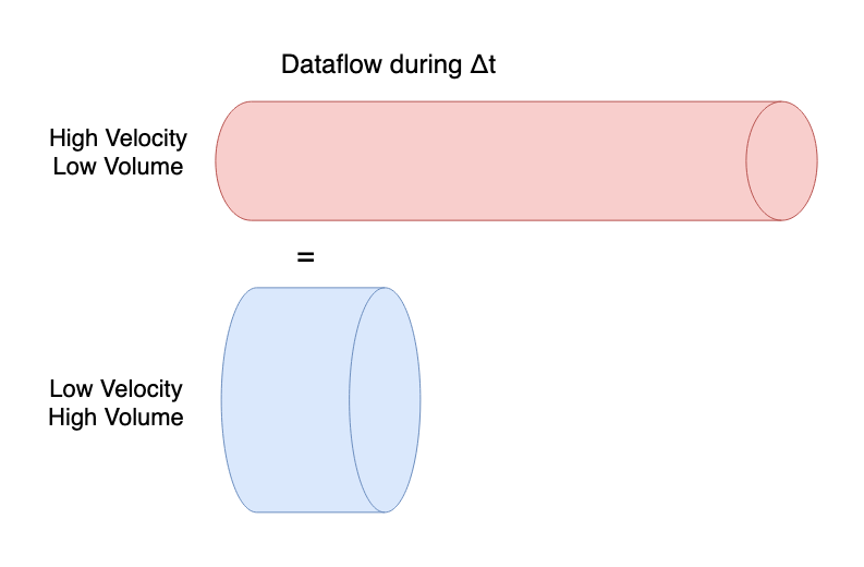
In some instances certain processes may not decrease the total data pressure but simply exchange one type of pressure for another. For example, batch processing may be slower, but will allow for processing much higher volumes efficiently, whereas you can avoid processing larger volumes by simply micro batch or stream processing at lower frequencies. One is not better than the other, one may simply be more strategically convenient than the other when you take the whole picture into account.
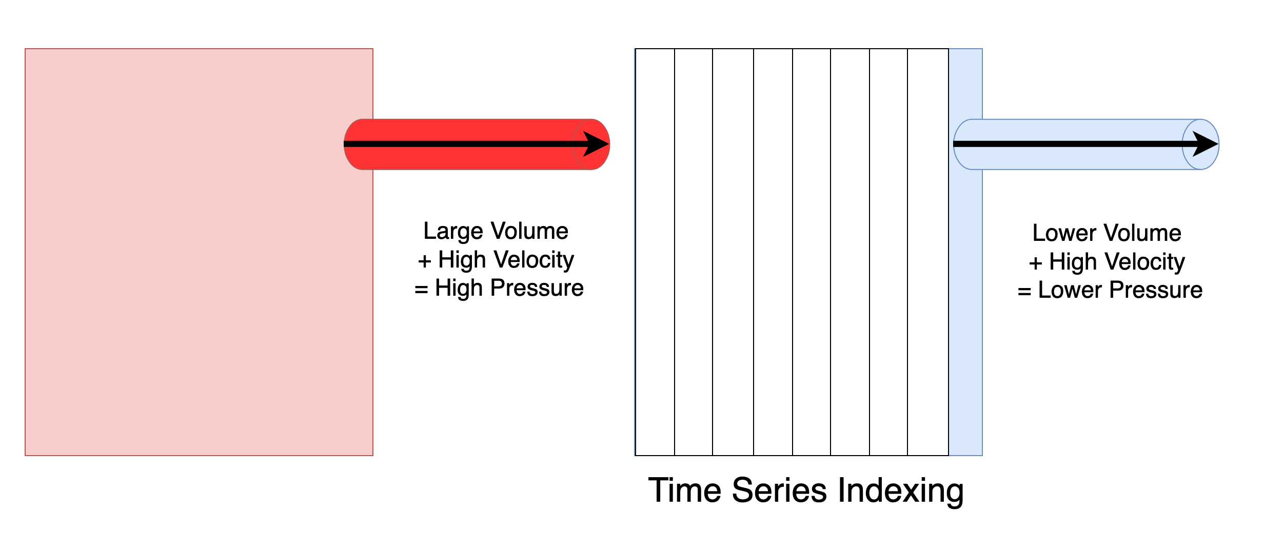
The other useful aspect of thinking in terms of pressure is that you can also think in terms of pressure differentials, for example, suppose that you have a very large dataset which you need to query with low latency. In this case the pressure differential between those two parts of the system is very large so you need to engineer vertical scaling or other strategies in order to lessen the effect of that pressure burden (i.e., don’t blow the valve on the other side), but if you find out that you only ever access a recent segment of the data then you can leverage a time series index or database, and now the pressure differential is much lower.

When thinking about data in terms of pressure a useful analogy of data to water comes to mind. In this way you can think about good data engineering much in the same way you would think of good plumbing. For example, a load balancer has a lot of similarities to a pressure balance valve, or a reducer is similar to a throttled producer. The goal of good data engineering in this regard simply is a matter of cutting up the data using horizontal scaling or other means such as denormalized stream consumers so no one component or machine is processing more pressure than it was designed to handle. Another tool in your toolbox is to simply “get a bigger machine”, or vertical scaling, however, when talking about many big data systems you have to be very careful about when you chose vertical over horizontal scaling because it is very likely you could get pinned into a corner, or become very dependent upon a large machine setup without a good strategy to move beyond it. Cost also becomes a big consideration when talking about vertical scaling.

An even better analogy than plumbing is roadway traffic engineering. Because a 7 lane highway you can think of in much of the same way as a 7 node compute cluster, each lane with its own respective capacity, and with costs associated with shuffling data (and thus cars) between the lanes. There are also many similar phenomena in traffic engineering where cascading effects can have unexpected effects, or in other words scaling up one part of a system may counterintuitively decrease the total system performance or bottleneck other parts of the system. IE, it doesn’t work to dump a 7 lane highway network into a sleepy neighborhood with two lane roads without some intermediate pieces to syphon off some of that traffic first and lesson the total “traffic pressure” it would exert on that neighborhood.
Variety
Variety is a broad and essential category in data engineering, that many are tempted to put too much de-emphasis on at the sake of the first two. There are many considerations but the main ones I will consider here are: flexibility, discoverability, and usability.
Flexibility
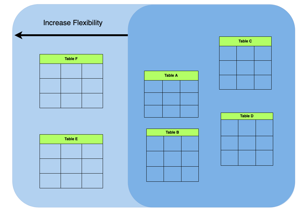
Flexibility expresses how quickly you system is able to adapt to new requirements. For example, you need to create a new table or index to express some new facet of a user population, but doing so in a conventional way may take too long. Or perhaps you need to filter or to facet the data in a new way or construct a complex view on the data totally ad hoc. Flexibility can also express the variety of data formats, for example, you need to process 3 data sources in json, another 6 in Parquet, another in Orc and one more in XML.
Flexible data strategies are strategies that take into account unknowns in business data needs and factor those unknowns explicitly in as dimensions and parameters to the data architecture. Flexibility, however, is not a good in itself to be pursued relentlessly to the abandon of other considerations. As with most things in software it comes at a cost, and a completely flexible “boil the ocean” type data strategy is likely to make tradeoffs for either performance or implementation time.
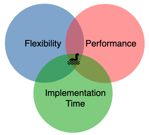
Working with companies to specifically address which dimensions of flexibility in a data strategy are mission critical and which are simply “nice to have” is very important as companies often overvalue some ancillary value adds without realizing the sometimes dramatic tradeoffs that may have with other more essential needs.
The strategy of “data denormalization” plays heavily into flexible data strategies as it allows you to create isolated “paths” of data pipelines which can be tailored towards certain specific use cases without having it tightly coupled to other previous data pipelines that may be geared towards totally different needs. In other words, denormalization allows you to create new data pipelines that are “blank slates” and don’t have to answer to the needs of other applications and use cases unnecessarily.
As time has gone on companies have started to fall back to creating these data pipelines rapidly and ad hoc on purely unstructured data by using a combination of in memory compute engines like Apache Spark in conjunction with materializations with query efficient storage formats like Apache Parquet as it allows them to exchange expensive and sometimes hard to maintain database migrations and indexes for simple denormalized derived data sets that can be deleted and rebuilt in various ways in isolation without affecting any other part of the data pipeline. In reality however, both a solid data warehousing SQL as well as unstructured data processing story are needed in a comprehensive data strategy.
Discoverability
Whereas flexibility defines the size of the cutting board a company has at its disposal when cooking data recipes, Discoverability defines the sharpness of its knife. Data that is discoverable is one that can be profiled in various ways in a purely ad-hoc fashion in order to gain insight into new dimensions worth investigating in the data. Discoverability is mostly discussed in the context of “data science enablement” or other higher-level analytics. Discoverability is a function of flexibility, ie the more flexible your data is, the more discoverable it naturally is going to be, but discoverability also expresses things like the ability to structure queries on the data that may have large data footprints and for those to be able to execute without crashing your query engine, or returning in a period of time larger than the age of the universe. Therefore, where flexibility defines the realm of what’s possible, discoverability defines the realm of what’s achievable and practical.
Any SQL on Hadoop style query engine such as Presto or SparkSQL are geared towards discoverability as they allow you to interact with big data in a way that is familiar to those do analytics on traditional data warehouses via SQL. Even tools like Zeppelin or Jupyter notebooks tied natively into Spark or Dask compute engines using tools like Spark magics or Dask Gateways can go a long way towards discovery by providing data scientists tools that are familiar to their workflow without sacrificing the aspect of scalability.
Useability
Useability expresses how ready the data is to be consumed whether its by a person, visualization software, or another software component or system. Big Data pipelines often take into account the heavy lifting or the most challenging aspects of a data architecture first as to eliminate the most risk from the overall plan of attack, but they sometimes leave a last bit of “connecting tissue” or what’s sometimes referred to as “last mile ETL” in connecting the heavy lifting to integrating pieces such as API integrations or webhooks. Other aspects of useability include security concerns such as encryption and decryption and delivery of data. Its important to think about the entire life cycle of data to determine if some pieces of the pipeline can truly be treated as a post hoc add on or last mile ETL, or if there is some major consideration hiding within those seemingly innocuous details.
Veracity
Veracity basically expresses “how do you know what is there is correct”. While for many companies large aspects of veracity fall out of the realm of data architecture and into the realm of QA engineering, many aspects of veracity can be alleviated or circumvented altogether by having a deliberate plan of attack up front.
Traceability
The term of endearment in traceability is what’s called “data lineage”. The trend in recent years behind breaking apart data pipelines into small self contained data “microservices” has allowed companies a lot of flexibility in being able to control how they role out changes, but has often created a mess in trying to trace down where a particular change in the data has originated as it could have its source four five or more steps back in a workflow from where the error begins to manifest itself. What’s more, machine learning and other more advanced applications have caused us to adopt practices that sometimes have totally chaotic and non linear paths of evolution for the data, resulting in black boxes sometimes impossible to reproduce. The king in this realm is “metadata management” and having an upfront metadata strategy that defines key metrics of success, and threads to follow defining and exposing your data lineage to the highest level without imposing unnecessary burdens on those having to interact with or do further processing on the data. A couple of ideas that make this easier could be:
- Federated Data Access This encourages the data model to be fully modelled and interacted with consistently across an organization allowing the companies data lineage to emerge and avoiding keeping critical interactions with the schema from being hidden away in scripts and notebooks and language specific code only privy to certain individuals within the organization. Tools like Dremio achieve this by creating a “virtual” federated access by providing a SQL interface that executes analytical query over a number of different stores by using the Arrow in memory compute engine and Parquet materializations which serve similar to database indexing. Tools like Spark and Databricks can achieve similar results by using spark query pushdown optimization to various data stores.
- Immutable Data Access By copying your data and only destructively interacting with copies of your data you can more easily trace back changes to your data, especially as your data model evolves over time. Semantically versioning your code and tying this to versions of your data can help with traceability as well. This comes at the cost of duplication of data, but can make tracing your data lineage and debugging issues dramatically easier. An example of a database that focus on this aspect specifically is Datomic
Explainability and Auditability
Explainability is a relatively new term in the world of machine learning models but nonetheless is pretty important. Machine learning models can sometimes function like a black box, in which the inner workings of trained models are hard to parse. Recently attention has been brought to the challenges this presents to QA and reproducibility of results and as a result several companies like Pachyderm and Fiddler have started to tackle this problem head on.
Auditability of data may relate to security and governance concerns, therefore having things like data access logs can become more important in some contexts.
Security
Security is too broad to go into any great detail here but suffice it to say it does play a factor. Mainly in plays a factor in the first golden rule of data security:
Don't ask for access to any data that you don't need to have accesss to
Many “data lakes” break this rule fundamentally by serving to basically collect as much data as possible without any plans or intentions about using it. Oftentimes the very idea of “data lakes” are antithetical to the idea of rigorous data engineering, and what you should actually be shooting for are interconnected isolated “data ponds”. However, oftentimes this doesn’t matter too much as long as you are not collecting “secure data”. Which brings me to the second golden rule of data security:
Don't ask for access to PII or secure data unless ABSOLOUTELY necessary
In other words, ask for deidentified, hashed, or pseudonymized data whenever possible. The number of parties responsible for secure data should be as absolutely small as possible to minimize the vectors for attack. If its possible to shift the responsibility of secure data to a (trustworthy) third party then you should always chose to do so.
Conclusion
This blog post was intended to be written for a mixed technical and generalist audience therefore it goes into varying level of details. These rules though not written in stone I have found are a good guide a lot of successful data engineering engagements. If this process sounds compelling to you Contact Us, we’d love to work with you!
Kyle Prifogle
